Sampling from Gompertz processes

TA Trikalinos

2025-08-20

Simulation description

Assume a population of $K = 10^{5}$ individuals indexed by $k \in [K] := \{ 1, \dots, K\}$. We will sample events from Gompertz processes over the age (time) interval $[T_{k0}, T_{k1})$. For example, $T_{k0}$ may be the age in years when person $k$ enters the simulation, and $T_{k1}$ the age in years when that person exits the simulation (e.g., dies from an ‘other cause’). (In practice, $T_{k1}$ would be obtained by separate point process.) Only some people will develop clinical cancer over their simulated lifetime.

To fix a simulation scenario, let $T_{k0} = 20$ for all $k$ and $T_{k1} \sim U(60 , 100)$, where $U()$ is the uniform distribution.

Setup

We will use data.tables – but the same analysis should be obvious in base R. We will use functions from three more packages, without loading them: The tictoc() package will be used for a simple time comparison between the different ways one can simulate this problem. The stats package is used to generate normally and uniformly distributed samples.

library(data.table)
library(nhppp)

Setup pop, the population data.table. The person specific values T_{k0}$ and $T_{k1}$ are variables in pop.

pop <- setDT(
  list(
    id = 1:K,
    T0 = rep(20, K),
    T1 = stats::runif(n = K, min = 60, max = 100)
  )
)
setindex(pop, id)
pop
#> Index: <id>
#>             id    T0       T1
#>          <int> <num>    <num>
#>      1:      1    20 95.12126
#>      2:      2    20 61.79684
#>      3:      3    20 99.27175
#>      4:      4    20 90.76692
#>      5:      5    20 61.40517
#>     ---                      
#>  99996:  99996    20 69.09209
#>  99997:  99997    20 74.66979
#>  99998:  99998    20 84.32928
#>  99999:  99999    20 98.94195
#> 100000: 100000    20 80.85864

The Gompertz Process functions

The Gompertz intensity function is

$\lambda_k(t) = a_k b_k \ e^{b_k t}$,

where $t$ is age in years. The parameters $a_k, \b_k$ are random over the individuals in the population with $a_k \sim U(0.0045, 0.0055)$, and $b_k \sim U(0.085, 0.095)$.

Add these values as person-level parameters in the dataset:

pop[, `:=`(
  a_gompertz = stats::runif(n = K, min = 0.0045, max = 0.0055),
  b_gompertz = stats::runif(n = K, min = 0.085, max = 0.095)
  )]

A cumulative intensity function is

$\Lambda_k(t) = a_k (e^{b_k t} - 1)$,

with the integration constant was arbitrarily set so that $\Lambda(0) = 0$. The inverse cumulative intensity function is

$^{-1}(z) = b_k^{-1}  ( -1 ) $.

Vectorized specification of the Gompertz $\lambda()$, $\Lambda()$, and $\Lambda^{-1}()$

Define vectorized forms of the Gompertz $\lambda()$, $\Lambda()$, and $\Lambda^{-1}()$ functions that take as default the values in pop.

l_gompertz <- function(t, a = pop$a_gompertz, b = pop$b_gompertz, ...) {
  a * b * exp(b * t)
}

L_gompertz <- function(t, a = pop$a_gompertz, b = pop$b_gompertz, ...) {
  a * exp(b * t) - a
}

Li_gompertz <- function(z, a = pop$a_gompertz, b = pop$b_gompertz, ...) {
  log(z/a +1) / b
}
 

Method 1: Vectorized sampling using only $\lambda()$

When you only know the intensity function $\lambda$, nhppp employs a thinning algorithm.

One of the items needed for the thinning algorithm is a piecewise constant majorizer function $\lambda_*$ such that: $\lambda_*(t) >= \lambda(t)$ for all $t$ of interest.

The nhppp::vdraw_intensity function assumes that you will provide the majorizer function as a matrix (lambda_maj_matrix). To create this matrix, split the simulation time (here, from age 40 to age 100) in $M$ equal-length intervals. For person $k$ and interval $m$, the element lambda_maj_matrix[k, m] records a supremum of $\lambda_k$ over the $m$-th interval. Any supremum will do – but the algorithm is most efficient when you give it the least upper bound – practically, the maximum of $\lambda(t)$ over all $t$ in the interval. For monotone intensity functions, such as the Gompertz, the maximum is at one of the interval’s bounds. It will be at the left bound, if $\lambda$ is decreasing, and at the right bound, if $\lambda$ is increasing.

There is a helper function in nhppp that generates the majorizer matrix automatically for monotone (and possibly discontinuous) functions and for nonmonotone continuous Lipschitz functions (functions whose maximum slope is bounded). Even if your case is more complex, you should be able to find a supremum that works.

This code samples in a vectorized fashion when you know only $\lambda()$. It creates a majorizer matrix over $M=5$ intervals (we chose this arbitrarily – not trying to be fast). To let the software know which times correspond to each of the $M$ intervals it suffices to specify a start and stop time for each row of the majorizer matrix with the rate_matrix_t_min and rate_matrix_t_max options. The sampling intervals $[T_{k0}, T_{k1})$for each simulated person are a subset of the interval for which the majorizer matrix is defined, and are specified with the t_min and t_max options. (The atmostB option can be useful to speed up the sampling and minimize memory needs when one is interested in the first event only. The smaller the value, the faster the algorithm but you have to check that you have not specified it to be too small. In this example, atmostB = 5 is fine – it returns exact solutions; but we have checked it [not shown]. If you do not want to mess with it, do not use the option. The function may be already fast enough for your needs).

tictoc::tic("Method 1 (vectorized, thinning)")
M <- 5
break_points <- seq.int(from = 20, to = 100, length.out = M + 1)
breaks_mat <- matrix(rep(break_points, each = K), nrow = K)

lmaj_mat <- nhppp::get_step_majorizer(
  fun = l_gompertz,
  breaks = breaks_mat,
  is_monotone = TRUE
)

pop[
  ,
  t_thinning := nhppp::vdraw_intensity(
    lambda = l_gompertz,
    lambda_maj_matrix = lmaj_mat,
    rate_matrix_t_min = 20,
    rate_matrix_t_max = 100,
    t_min = pop$T0,
    t_max = pop$T1,
    atmost1 = TRUE,
    atmostB = 10
  )
]
tictoc::toc(log = TRUE) # timer end
#> Method 1 (vectorized, thinning): 0.227 sec elapsed

Method 2: Vectorized sampling using $\Lambda()$ and $\Lambda^{-1}()$

The most efficient sampling is possible when one knows $\Lambda()$ and $\Lambda^{-1}()$. The nhppp package can sample in this case using the vdraw_cumulative_intensity() function. Here range_t is a matrix with information on each person’s $[T_{k0}, T_{k1})$.

tictoc::tic("Method 2 (vectorized, inversion)")
pop[
  ,
  t_inversion := nhppp::vdraw_cumulative_intensity(
    Lambda = L_gompertz,
    Lambda_inv = Li_gompertz,
    t_min = pop$T0,
    t_max = pop$T1,
    atmost1 = TRUE
  )
]
tictoc::toc(log = TRUE) # timer end
#> Method 2 (vectorized, inversion): 0.008 sec elapsed

Comparisons

Simulation time-costs

The simulation time-costs that you see in this document depend on the machine that rendered it. If you read this online, this machine is probably some virtual server with minimal resources. If you installed the package locally, it is probably the machine you are using to run R.

1. Method 1 (vectorized, thinning): 0.227 sec elapsed. This is the slower approach – but still not bad for $10^{5}$ samples! It uses the thinning algorithm which is very flexible – it can accommodate very complex time varying intensity functions. You almost always know $\lambda$ and can get its majorizer $\lambda_*$ easily and fast.

2. Method 2 (vectorized, inversion): 0.008 sec elapsed. This approach is many times faster that the previous one, but requires implementations for $\Lambda$ and $\Lambda^{-1}$.

Simulated times

Both methods sample correctly from the specified Gompertz process. There is no approximation at play.

The QQ plots compare the simulated times with the two methods. The agreement is excellent over this population of size $K = 10^{5}$. As $K$ increases the agreement remains excellent (not shown here - try it for yourself). The paper in the bibliography includes in-depth comparisons. A set of QQ plots should suffice here.

qqplot(pop$t_thinning, pop$t_inversion)

Simulating all event trajectories

In the above, we simulated the time to first event. Let’s simulate all times that realize from that process in the interval of interest. You can use either method; we demonstrate with the faster one.

Z <- nhppp::vdraw_cumulative_intensity(
    Lambda = L_gompertz,
    Lambda_inv = Li_gompertz,
    t_min = pop$T0,
    t_max = pop$T1,
    atmost1 = FALSE
  )

dim(Z) # a lot of events!
#> [1] 100000     87

There is at least one person among the 10^{5} simulated persons with 87 total events in the interval of interest.

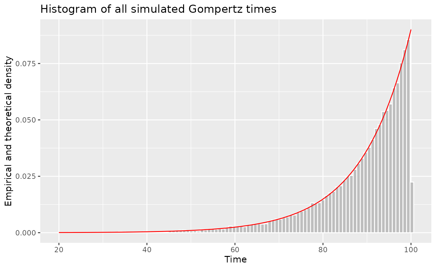
Demonstrating that we simulate from the correct intensity function

Let’s fix the parameter values for all $K$ people and do a histogram of the simulated times. They match the shape of the intensity function over the interval $[T_0, T_1)$, scaled to unit area, i.e. $\frac{\lambda(t)}{\big(\Lambda(T_1)-\Lambda(T_0) \big)}$. Run more samples to convince yourself – or also calculate the Wasserstein distance of the empirical and theoretical distribution, as described in the numerical analyses in the nhppp paper.

if(nchar(system.file(package = 'ggplot2'))>0) {
  pop2 <- setDT(list(id = 1:1000)) 
  pop2[, `:=`(
    T0 = 20, 
    T1 = 100, 
    a = 0.005, 
    b = 0.090
  )]
  setindex(pop2, id)
  pop2
  
  ## re-define functions to use `pop2` by default 
  ##    clunckiness of `nhppp` -- help us improve it!
  l  <- function(t, a = pop2$a, b = pop2$b, ...) a * b * exp(b * t)
  L  <- function(t, a = pop2$a, b = pop2$b, ...) a * exp(b * t) - a
  Li <- function(z, a = pop2$a, b = pop2$b, ...) log(z/a +1) / b
  
  ## get all times (full trajectories)
  Z <- nhppp::vdraw_cumulative_intensity(
      Lambda = L,
      Lambda_inv = Li,
      t_min = pop2$T0,
      t_max = pop2$T1,
      atmost1 = FALSE
    )
  
  ## ignore non-realized times 
  Z <- as.vector(Z)
  Z <- Z[!is.na(Z)]
  
  x <- seq(from = 20, to = 100, length.out = 100)
  ## normalize the hazard rate to have area 1 between 20 and 100
  y <- l(x, a = pop2$a[1], b = pop2$b[1]) / (
        L(100, a = pop2$a[1], b = pop2$b[1]) - 
        L(20, a = pop2$a[1], b = pop2$b[1])
       )
  
  
  library(ggplot2)
  ggplot(xlim = c(0, 110)) +
    geom_histogram(
      aes(x = Z, y = after_stat(density)), 
      bins = 100, 
      fill = "gray", 
      color = "white") +
    geom_line(
      aes(x = x, y = y), 
      color = "red"
    ) +
    labs(title = "Histogram of all simulated Gompertz times", x = "Time", y = "Empirical and theoretical density")
}

Acknowledgments

Thanks to Fernando Alarid-Escudero for suggesting this vignette.

Bibliography

Trikalinos TA, Sereda Y. nhppp: Simulating Nonhomogeneous Poisson Point Processes in R. arXiv preprint arXiv:2402.00358. 2024 Feb 1.

Trikalinos TA, Sereda Y. The nhppp package for simulating non-homogeneous Poisson point processes in R. PLoS One. 2024 Nov 21;19(11):e0311311.

Marshall AW, Olkin I. “The Gompertz distribution” (p 364) in Life distributions Springer, New York; 2007.

Since the publication of the paper, the syntax and options of the nhppp package have evolved. To reproduce the code in the paper, you have to install the version of nhppp used in the paper. Alternatively, take a look at the vignettes, which are written to work with the current package.